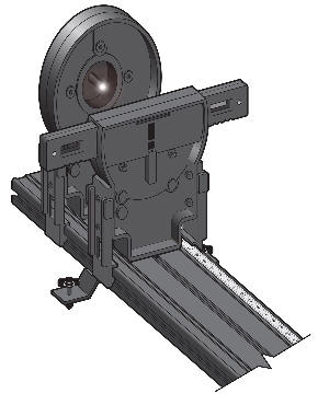
Laser and Slit Assembly
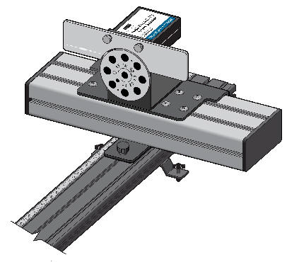
Light Sensor Assembly
Interference
As long ago as the 17th century, there were two competing models to describe the nature of light. Isaac Newton believed that light was composed of particles, whereas Christopher Huygens viewed light as a series of waves. Both models could explain reflection and refraction, but the phenomena of diffraction and interference could be more easily explained by Huygens’ wave model. In the early 19th century, Thomas Young’s double-slit experiment provided evidence that supported the wave nature of light. You will explore single and double-slit interference patterns.
Direct exposure on the eye by a beam of laser light should always be avoided with any laser, no matter how low the power.
1.If not already in place, attach the laser at one end of the track so that it faces down the length of the track. Connect the power supply. Leave the laser off until all parts are in place to avoid accidental reflections. Place the diffraction slit assembly on the track near the laser as shown in the sketch below.
|
|
|
|
Laser and Slit Assembly |
Light Sensor Assembly |
2. Set the diffraction slit assembly to a single slit of width, a = 0.08 mm. If not already in place, attach the assembly to the track, with the silver reflective side of the glass plates facing the laser. Position it about 10 cm from the laser assembly.
3. If not already in place, attach the High Sensitivity Light Sensor and the Linear Position Sensor to the other end of the track, with the light sensor facing the slits.
4. Turn on the laser. Adjust the horizontal laser position to achieve maximum brightness of the pattern. Adjust the vertical laser position to center the pattern vertically on the entrance aperture of the light sensor. Use this procedure every time you change the slits. Slide the light sensor assembly so that the pattern from the beam falls on the screen to one side or the other of the aperture disk (see Figure above).
5. Observe features of the pattern and record your observations in your lab notebook.
6. Now, set the slit assembly to a double slit where the slit width, a, is 0.08 mm, and the slit separation, d, is 0.25 mm. Align the laser as you did in Step 4.
7. View the pattern that forms as the laser beam passes through the double slit. Describe your observations in your lab notebook, then turn the laser off.
Discuss what features the patterns have in common and the ways they appear to differ. You may find it helpful to repeat your observations of the single slit and double slit patterns.
8. Return to the diffraction apparatus. Examine the pattern obtained when the laser shines through the single slit with a = 0.08 mm. Using a ruler, measure the distance between the midpoint of the central bright region and the midpoint of the first dark fringe. Repeat this measurement for the second dark fringe. Then, measure the width of the central bright region from dark fringe center to dark fringe center.
9. Now, take a closer look at the pattern obtained when the laser shines on the double slit used in the Pre-Lab Investigation (a = 0.08 mm, d = 0.25 mm). Using a ruler, measure the distance between the middle of the central bright region and the location where the alternating bright and dark fringes seem to disappear. Then, measure the width of the central bright region.
10. Compare your measurements for the single- and double-slit patterns. What feature of the pattern appears to arise from the single slit? What feature appears to arise from the double slit?
11. Consider what feature of the single-slit pattern would change if you changed the slit width. Test your prediction. Record your observations.
12. Consider what feature of the double-slit pattern would change if you used the same slit width but changed the separation between the slits. Test your prediction. Record your observations.
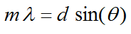
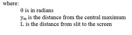
The double slit pattern discovered by Young is described by the equation below. m is an integer (0 for the central maxima, +1 for the first maxima to the right, -1 for the first maxima to the left, etc), d is the slit separation and theta is the angle light to that maxima makes relative to the path for m = 0. Units should be SI for least confusion.
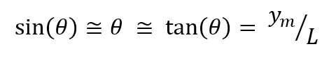
In the case of small angles - which occur when L >> ym, one can use the small angle approximation given below, where ym is the distance to the side away from m = 0 and L is the distance from the slit to the detector.
13. If not already connected, connect the High Sensitivity Light Sensor and the Linear Position Sensor to the interface to the Lab Pro and start Logger Pro.
14. Record the distance, L, from the slit assembly to the light sensor. Record the slit width, a, and the slit separation, d, for the double-slit configuration you used in Part 1, as well as the wavelength of the laser.
15. The optimal combination of light sensor sensitivity and sensor aperture depends on the type of laser and the slit configuration. It allows an intensity reading that reveals the detail necessary for you to make your measurements. For the red laser and the double-slit configuration you used earlier, we suggest setting the sensitivity to 10 microwatts and using an aperture of 0.5 mm.
16. Move the sensor assembly all the way to the right as viewed from the laser. Zero both sensors.
Do not move the sensor assembly stage between runs or the second run will be shifted horizontally!
17. Start data collection, and then move the sensor assembly stage toward the other side of the rail on which it is mounted. Take at least 20 seconds to execute the motion, slowing when the sensor is traversing the brightest portions of the pattern. Stop collecting data when the stage reaches the end stop. Test that you moved the stage sufficiently smoothly by storing the run and collecting another run, moving the stage in the opposite direction. The trace of the second run should overlay that of the first.
18. Choose a double-slit configuration in which you change either the slit width or the slit separation, then repeat the previous step (be sure to store your runs when you have clean data). You may find it necessary to change the aperture on the light sensor to obtain sufficient detail to complete your evaluation of data. When you are finished collecting data, save your experiment file and turn off the laser.
Analysis
19. Start a table in your notebook with the following columns:
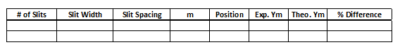
a). View the intensity vs. position graph for your first trial. Zoom in on the portion of the graph that shows the most useful information. Choose the Examine tool from the Analysis menu and position the cursor on the peak corresponding to the central maximum. Record the position in your table (m = 0) .
b) Repeat for the bright fringes on either side of the central maximum. If you have difficulty finding the m = 3 bright fringe, explain why.
c). Determine the distance, ym, from the central maximum to each of the fringes on either side. (Remember distance is always positive while m can be either positive or negative) If the distances are not the same on either side for a given value of m, decide how to best report them.
d). From the values of L, d and wavelength, calculate the theoretical distance ym, for each value of m (other than zero) in your table. The agreement between theory and experiment should be reasonably good. If not, check for mistakes in your computations - not SI units, didn't use the distance, wrong value of m, etc.
e). Determine the percent difference between the theoretical and experimental values of the fringe spacing for this double-slit configuration.
f). Repeat Steps 'a' - 'd' for trials you have performed with other double-slit configurations. Please leave an empty row between different slit configurations. If more than two bright fringes are detectable, measure the positions at least three of them.
g). How would your table be different if you were to repeat the experiment using a green laser that has a significantly shorter wavelength?
Reflect on the results in your table. What have you learned about interference and diffraction.