 |
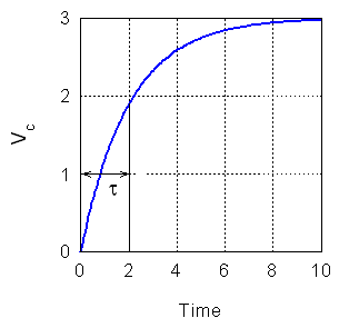
| Figure 1. Voltage of a charging capacitor |
RC Circuit and its Time Constant
When a resistor, capacitor and battery are connected in series, the current is initially large and has a value Vo/R. As the capacitor gradually charges, the current decreases. When the capacitor is fully charged (the capacitor voltage is equal to the battery voltage), the current is zero. The process of the current going from its maximum value to zero is an exponential decay. We characterize this process by the "time constant" of the circuit. At the time t = RC the capacitor will be charged up to approximately 2/3 (or 1-1/e exactly) of its final value. This time is referred to as the time constant of circuit. The charging process is illustrated in the figure below showing a graph of capacitor voltage versus time. A graph of the charge on the capacitor would have the same shape since Q = C V.
|
| Figure 1. Voltage of a charging capacitor |
Time constants tend to be small, and until recently, it was very difficult and very expensive to capture the charging (or discharging) of a capacitor. Historically an oscilloscope and a square-wave function generator have been used to measure time constants. The oscilloscope displays a plot of V vs. t, and the repetitive signal from the function generator continually charges and discharges the capacitor which causes the screen to be refreshed so the display will remain bright. A square-wave is a wave that has a value of Vm for half of its period and zero for the other half of the cycle. Not shown in the diagram above is what happens when the signal drops to zero for the second half. The voltage across the capacitor decreases exponentially to (almost) zero and then the process repeats.
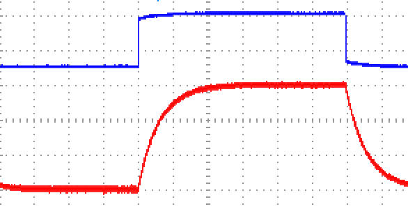
In our lab we want to scale the voltage to be either 3 or 6 blocks tall from zero to Vm so that we will have lines on the screen at 2/3 Vm. It is very important that the voltage be essentially flat in the time before the function drops to zero. Otherwise, we will have a systematic error in our calculations that cannot be easily corrected for. The following graph indicates what you need in terms of flatness before the change. Notice that the corners of the 'square' wave are rounded off. The graph shows the square-wave displayed at 2.0 V/div and the voltage on the capacitor at 1.0 V/div. The function generator is set for 3.0 Vpp, and the voltage on the capacitor has been shifted until the zero level is 2 divisions below the center of the screen. The smaller square-wave has been shifted up, so that it is still visible, but does not interfere with the measurement of the time constant.
The time constant is the time that elapses between when the capacitor starts charging and the voltage across the capacitor is 2/3 of the voltage from the function generator. We can use the vertical segment in the square-wave as our t=0 time. The Horizontal Position can be used to shift both curves right or left - until the vertical line is on a grid line. If you look at the red curve, you will see that the time constant is about 0.6 divisions multiplied by the Time/Div. However, the uncertainty is huge. We want to expand the horizontal scale so that the rise to 2/3 of the final value takes several divisions. Doing so will greatly reduce the error bars on the resulting time constant.
|
| Figure 2. Necessary shapes to obtain accurate data. |
PROCEDURE:
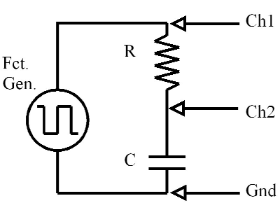
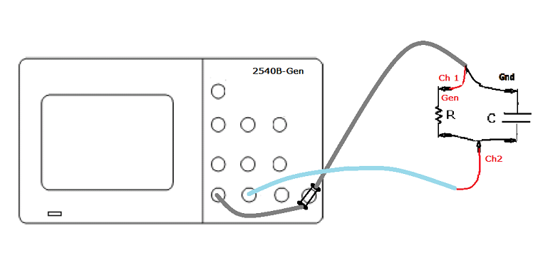
Since Channel 1 always measures the generator voltage, we will use a 'Tee' on the generator and connect one side to Channel 1and the other end to the circuit as shown in the pictorial. If the cable connected to Channel 2 has a black (ground) alligator clip, fasten it to the rubber of the cable to keep it from inadvertently shorting out part of the circuit.
| Set the Function Generator to output to a square wave |
| Press 'Menu' on the function generator |
| Press the 'Soft Key' beside 'Output Type' |
| If not 'Square' then rotate the knob to select 'Square' and then 'Press and Release' the knob. |
| Set the frequency to 500 Hz |
| Press the 'Soft Key' beside frequency - if the frequency is not 500 Hz then follow the steps below |
| Press the arrows to get to the most significant digit |
| Rotate the knob to select 5 |
| Press the arrow to the right and set the digit to zero |
| Repeat the previous step until the first three digits are 500 |
| Move the arrow to the right until the units below the number are red |
| Rotate the knob until the frequency shown is 500 Hz or 0.500 kHz |
| Press and Release the knob. |
| Next we will set the amplitude to 3 Vpp and turn the output 'On' |
| Press the 'Soft Key' beside 'Ampl' |
| Follow the same steps as you did for the frequency until the setting
shows 300 for the most significant digits. |
| Move the arrow to the right until the units below the number are red |
| Rotate the knob until the display shows 3.00 Vpp |
| Press the 'On/Off' button just above the 'Gen' cable to turn the output
on. |
| R = 3.3 x 10⁴ ohms and C = 0.001 µF |
| R = 2.7 x 10⁵ ohms and C= 100 nF |
| R = 1.5 x 10⁴ ohms and C = 0.1 µF |
| R = 2.7 x 10³ ohms and C = 0.05 µF |
Correction of a systematic error
The approximation where we used 2/3 of the maximum voltage to find the time constant has a systematic error. It tends to overestimate the time constant - by the same factor for all measurements as shown in the figure below.
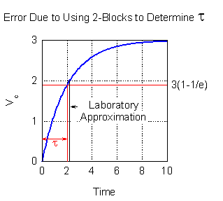
Calculate the quantity 3(1-1/e) [or the quantity 3(1-e-1) if that is easier to enter into your calculator] and record it in your notebook. The value should be less than 2.0. Divide that number by 2. This is the correction factor that will reduce your approximate experimental time constant to the best experimental value. Make a table in your notebook with the following columns: R, C, tapprox, texp, and ttheory. The theoretical time constant is the product of the measured resistance and the printed capacitance.
When completing your write-up, you may wish to make a graph of Experimental Time Constants versus Theoretical Time Constants. Ideally, the graph would be a line of slope 1 that passes through the origin. Any errors due to miscalculation or mistakes in reading would prominently show on the plot.