 |
| Figure 1. Voltage of a charging capacitor showing the time constant. |
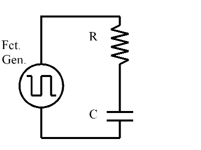
RC Circuit and its Time Constant
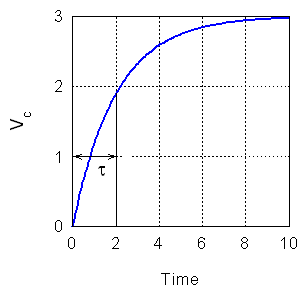
When a resistor, uncharged capacitor and battery are connected in series, the current is initially large and has a value Vo/R. As the capacitor gradually charges, the current decreases. The uncharged capacitor has a voltage of zero. When it is fully charged (the capacitor voltage is equal to the battery voltage), the current is zero. As the capacitor discharges, the process of the voltage going from its maximum value to zero is an exponential decay. We characterize this process by the "time constant" of the circuit. At the time t = RC the capacitor will be charged up to approximately 2/3 (really 1-1/e or about 63%) of its final value. This time is referred to as the time constant of circuit. The charging process is illustrated in Figure 1 below showing a graph of capacitor voltage versus time. A graph of the charge on the capacitor would have the same shape since Q = C V. Notice how the thick line indicating the time constant rises up almost to 2/3 of the battery voltage.
|
| Figure 1. Voltage of a charging capacitor showing the time constant. |
The discharge of the capacitor is shown in Figure 2. In this case we are going to approximate the time constant by the amount of time that it takes the voltage to drop to 1/3 of its maximum value. As you can see, this is a slightly longer time, but it offers an advantage of quickly measuring the time constant using the DSO. It turns out that the approximate time constant can be easily corrected as we will see later.
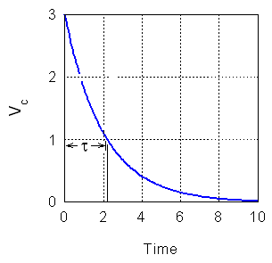 |
| Figure 2. Voltage of a discharging capacitor showing the approximate time constant. |
Time constants tend to be small, and until recently, it was very difficult and very expensive to capture the charging (or discharging) of a capacitor. Historically an oscilloscope and a square-wave function generator have been used to measure time constants. A square-wave is a wave that has a value of Vm for half of its period and zero for the other half of the cycle. The oscilloscope displays a plot of V vs. t, and the repetitive signal from the function generator (changing from zero to a maximum with a constant period) continually charges and discharges the capacitor which causes the screen to be refreshed so the display will remain bright. Figure 1 is the charging portion of the square wave and Figure 2 is the discharge. Together they would show one complete cycle.
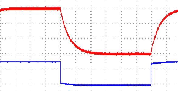
In our lab we want to scale the voltage to be either 3 or 6 blocks tall from zero to Vm so that we will have lines on the screen at 2/3 Vm. It is very important that the voltage be essentially flat in the time before the function drops to zero. Otherwise, we will have a systematic error in our calculations that cannot be easily corrected for. The following graph indicates what you need in terms of flatness before the change. Notice that the corners of the lower 'square' wave may be slightly rounded off, however, the regions just before the vertical transitions are horizontal. The graph shows the square-wave displayed at 2.0 V/div and the voltage on the capacitor at 1.0 V/div. The function generator is set for 3.0 Vpp, and the voltage on the capacitor has been shifted until the zero level is 1 divisions below the center of the screen. The smaller square-wave has been shifted down, so that it is still visible, but does not interfere with the measurement of the time constant.
The time constant is the time that elapses between when the capacitor starts charging and the voltage across the capacitor is 2/3 of the voltage from the function generator. We can use the vertical segment in the square-wave as our t=0 time. The Horizontal Position can be used to shift both curves right or left - until the vertical line is on a grid line. If you look at the red curve, you will see that the time constant is about 0.6 divisions multiplied by the Time/Div. However, the uncertainty is huge. We want to expand the horizontal scale so that the rise to 2/3 of the final value takes several divisions. Doing so will greatly reduce the error in the resulting time constant.
|
| Figure 3. Necessary shapes to obtain accurate data. |
PROCEDURE:
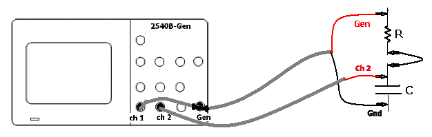
- If not already set up, connect the BNC 'Tee' to the generator output. Connect short dual BNC cable between 'Ch 1' and the 'Tee'. Connect a BNC cable with both red and black alligator clips to the BNC 'Tee' also. Use an alligator clip lead to connect the resistor to the capacitor. Connect the cable with two alligator clips to your circuit, making sure the black lead is connected to the free end of capacitor and the red lead to the free end of the resistor.
- Place the BNC cable that has only one alligator clip on 'Ch 2' and connect the clip to the junction of the resistor and capacitor as shown. 'Ch 2' is your experimental value channel.
- 'Ch 1'will measure the voltage being output by the generator (which may not necessarily be the same as the voltage that you set for the function generator due to possible overloading).
| Set up 'Ch 1' and 'Ch 2' and the Triggering |
| Press 'Ch 1' and then 'Coupling'. If it is not on 'DC' set it to 'DC' and turn the soft menu off. |
| Press 'Ch 2' and then 'Coupling'. If it is not on 'DC' set it to 'DC' and turn the soft menu off. |
| Set the 'Ch 1' sensitivity to 2 V/div and the 'Ch 2' sensitivity to 1 V/div. |
| Set the timebase to 5ms/division. |
| Press the 'Trigger' button, make sure the 'Source' is 'Ch 1' and 'Mode' is 'Normal' then turn off the soft menu. |
| Set the Function Generator to output to a square wave |
| Press 'Menu' on the function generator |
| Press the 'Soft Key' beside 'Output Type' |
| Rotate the knob to select 'Square' |
| Press and Release the knob. |
| Set the frequency to 200 Hz |
| Press the 'Soft Key' beside frequency |
| Press the arrows to get to the most significant digit |
| Rotate the knob to select 2 |
| press the arrow to the right and set the digit to zero |
| repeat the previous step until the first three digits are 200 (don't worry if there is a decimal point and ignore the other digits for now) |
| Move the arrow to the right until the units below the number are red |
| Rotate the knob until the frequency shown is 200 Hz or 0.200 kHz |
| Press and Release the knob. |
| Next we will set the amplitude to 3 Vpp |
| Press the 'Soft Key' beside 'Ampl' |
| Follow the same steps as you did for the frequency until the setting shows 300 for the most significant digits. (Ignore the decimal and any trailing digits) |
| Move the arrow to the right until the units below the number are red |
| Rotate the knob until the display shows 3.00 Vpp |
| Press the 'On/Off' button just above the 'Gen' cable to turn the output on. You should hear a 'click' and the button will be green. |
The approximation where we used 1/3 of the maximum voltage to find the time constant introduced a systematic error. It tends to overestimate the time constant - by the ratio of 36.8% to 33.3% for all measurements as shown in the figure below.
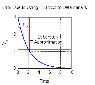
To correct for overestimating the time constant we need to multiply the approximate time constant we measured by 0.948. This is then the best value we can obtain experimentally for the time constant of the circuit.
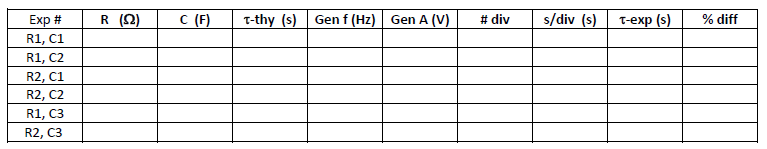
Enter your theoretical and experimental values of the time constant into Graphical Analysis or Logger Pro.
Add a calculated column whose values are 0.948 times the experimental time constant.
Plot a graph of the calculated column versus the theoretical time constant and perform a linear least squares fit.
If the data and calculations are good the slope should be approximately one with an intercept near zero.
If you have data points that fall far from the line, be sure to check for errors in those points before proceeding.
Comment on how your experimental results correspond to the predicted theoretical results.