Spectrum of Atomic Hydrogen

Adapted from "Spectrum of Atomic Hydrogen" in "Advanced Physics with Vernier – Beyond Mechanics" ©Vernier Software & Technology

Reading the Review of Bohr Theory is recommended before starting this experiment.

OBJECTIVES

In this experiment, you will:

Observe light sources through a diffraction grating.
Use a photodiode array spectrometer to make a qualitative investigation of the spectrum of several different kinds of light sources and categorize their spectrum as broadband continuum, narrowband continuum, line or composite.
Perform a quantitative study of the visible spectrum of hydrogen.
Determine the wavelengths of the emission lines in the visible spectrum of excited hydrogen gas.
Determine the energies of the photons corresponding to each of these wavelengths.
Use Bohr Theory to relate the photons’ energies to specific transitions between energy levels.
Use your data and the values for the electron transitions to determine a value for Rydberg’s constant for hydrogen and determine the lowest energy Bohr state for your hydrogen spectrum..
Compare your experimental value for the Rydberg constant to the accepted value.

Preliminary INVESTIGATION

1.  Plug in the straight-filament lamp. View the spectrum through the diffraction grating. When finished, remove power from the lamp. Describe in your notebook what you observed.
2. If necessary, rotate the carousel to place the hydrogen discharge tube in. Turn on the power and observe the bright line spectrum of hydrogen through the diffraction grating. Turn the power off (the hydrogen tube has a very limited lifetime). Record your observations.
3. Use your grating to look at the overhead fluorescent lights.
4. Discuss the differences in the spectra from these two sources.

Warning: Never touch the ends of the optical fiber and never allow the fiber to kink tightly.  The optical cables are fragile and easily damaged.

1. If it is not connected, connect the Vernier spectrometer to a USB port on the computer. Double Click ‘Spectral Studies.cmbl’ in the PHY 173 or PHY 183 folder, as appropriate, to Start Logger Pro. If not already connected, carefully connect the optical fiber cable to your spectrometer by removing the plastic protection sheath, inserting the bundle into the screw fixture on the spectrometer and gently tightening the outer shell until it is just snug.
2. Check settings for the ‘Spectral Studies’ experiment and adjust if necessary.
   1. Choose Change Units ►Spectrometer ►Intensity from the Experiment menu. The software will measure the intensity in relative units.
   2. Next, choose Set Up Sensors ►Spectrometer from the Experiment menu. Change the data-collection duration to 40 ms if it is not set already.
   3. Go to page 1: Qualitative. Check to see that the graph is set up with vertical divisions of 0.001, 0.01, 0.1 and 1.0.
      1. If not, right click on the graph, go to Graph Options, then axes and click the ‘Log axis’ box.
      2. Set the maximum value to 5 and the minimum value to 5E-4.
      3. This setting will compress the tall features on the graph allowing smaller features to be identified as being present. The value around 0.001 represents no light detected by the spectrometer.

Qualitative classification of light sources

Be sure to record the name of your light source in a table – i.e. green LED, helium tube, etc – as you take your data. Otherwise you will have a lot of curves but may not know what they are.

3. Point your fiber at the overhead fluorescent lights.
4. Click ►Collect to start the program taking data and position the optical fiber until you have a plot that is above 0.5 at its highest point but less than one. Stop the data collection. (The next time you click Collect, you will be asked if you want to store or discard the previous data – always choose to store unless you are repeating on the same lamp. Be sure to record the data name beside the light source you recorded earlier.)
5. If it is a sunny day, turn the room lights off and point your fiber at the windows and repeat step #4.
6. You have a bulb and two batteries and some wires. Make the bulb light. And repeat step #4. Disconnect the lamp when finished.
7. You have a box with three pushbuttons and a snap to a battery pack.  If not attached, place the snap on the connector of the battery holder that uses 3 "AA" batteries -Never connect the LED Box to a 9-volt battery! If you look on the side of the box there is a small hole that will show light when one of the buttons is pushed.  The hole is intentionally too small to be able to insert the optical fiber.  The LEDs are too bright for the spectrometer to measure them directly, so there is a 'process' involved:
• Click on 'Collect' in Logger Pro
• Hold the end of the fiber up to the hole and 'tilt' the fiber until a reasonably large spectra is observed.
• Click 'Stop' on Logger Pro to capture the spectrum.
• Label the curve in Logger Pro in the same manner you labeled the spectrum for the lamp.
Once you have completed all 3 colors, try taking a spectra of all 3 LED's at once. Is it the superposition of the three individual curves? Explain in your notebook.
• Set the LED box aside, beings sure that nothing is pressing on the buttons.
8. Your discharge lamp fixture (the green cylinder with the black carousel) has a bracket that will hold the end of the optical fiber in position relative to the lamp. Place the optical fiber in the notch and lightly tighten the screw on the hexagonal metallic part of the end of the fiber optic cable. Do not over-tighten. The carousel can be rotated (with the power off) to change light sources. The lamp can be gently rocked from side to side while on to better position the lamp and optical fiber if need be. Notes: Hydrogen tubes have a limited lifetime, so turn the tube off when you are not taking data. Air tubes may take several minutes to start.
9. For each of the lamps in the discharge carousel repeat step #4. You should have the intensity of the strongest line above 0.4 but no lines should be ‘clipped’ at the value 1.0 (or 10⁰ on the graph). If necessary, rock the carousel gently to change the amount of light entering the fiber. Turn the lamp off as soon as you stop data collection.
10. Save your experiment on the Desktop.
11. Change to page ‘2: No Color’ in Logger Pro which is the same graph without the color spectrum background.
12. Print a graph of your curves (without the data tables) and include in your lab report.
13. Classify the curves into the categories of line, broad continuum, narrow continuum, or composite - where composite exhibits line behavior superposed with a continuum.  Make a table in you notebook similar to the one below. Explain why you classified each curve as you did. The italicized items in the table are hints for you and need not appear in you table.  The bold headings or something equivalent should be present in your table.
    
    

    Source Name (as it appears in your notebook)	Classification:   (Continuous,    Line or Mixed)	Explanation (of why you chose that classification - you may need more than one line)

This completes the qualitative component of this lab.  Be sure to reflect in you lab notebook.

Quantitative analysis of the hydrogen spectrum.

Hide all of your curves except for the hydrogen spectrum. You should be able to see 4 or 5 peaks representing the location and intensity of the ‘spectral lines’. The most intense line should have an intensity less than 1.00. If this is the case you can use the data you have already taken. If not, you will need to acquire a new spectrum that shows 4 or, preferably, 5 peaks without clipping the most intense peak at a value of 1.00 (clipping refers to cutting the top off a curve, much like clipping a blade of grass while mowing). If you take new hydrogen data be sure to save your experiment file and to turn off the hydrogen discharge tube as soon as you finish.

EVALUATION OF DATA

 At this point, you should be on page '2: No Color' the only graph on your screen should be your hydrogen spectrum. If this is not the case, hide all of the other curves except for hudrogen before proceeding.

1. Use the Examine tool to find the center wavelength for the red line you observed in the H-spectrum. Record the wavelength in a table in your lab notebook like the one shown below. Repeat this step for the remaining peaks.  If you need to be reminded of color, refer to the first page.
2. Change to page ‘3: Rydberg’ in Logger Pro and enter your peak wavelengths in the appropriate column. The first line is a placeholder to keep the formula to convert the wavelength into photon energy - type over the values in that line. The photon energy for that wavelength will be calculated automatically (in eV) in the appropriate column. Copy those values for wavelength and change in energy into your data table in your notebook.



3. The photon energies calculated in Step B result from differences in the allowed energy states of the electron in hydrogen atoms, DE = E_final – E_initial. While they provide a clue to the allowed energy states, these values alone are insufficient to determine the actual energy of the allowed energy states. From Bohr Theory you know that the energy levels for a hydrogen atom are given by

   

    We can, however, make use of the fact that DE = hf = h(c/λ) to obtain a form of the Rydberg equation that relates the energy of the emitted light to the initial and final energy states in terms of photon energy in eV.

    

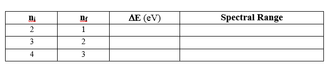
   Using Bohr's equation above, complete the table below and include it in your notebook. These are the lowest energy photons emitted for a given value of n-final.  The range of visible light is approximately 2 to 4 eV.  Compare your value for Delta-E to determine the spectral range as either infrared, visible, or ultraviolet.

   

4. From the preceding step, you now know the most likely value of n-final for you data.  Starting with the most red line and moving towards the blue in the specturm the value of n-initial must increase.  Return to page ‘3: Rydberg’  in Logger Pro and enter your values for n_i and l in the appropriate column in the table. (be sure to overwrite the first point in the table with your data otherwise the fit will not yield the correct value).  Logger pro will calculate the reciprocal wavelength and 1/n_i² and generate two plots: one for the equation in step 'C' and another for the classic Rydberg equation. Your points should fall along a straight line that slopes down. If you have curvature or significant outliers, re-check your value for n_i. Linear fits to the data on each graph are already set up.  You will need to change the values on the x-axis to make the line cover most of the plot.
5. Your slope on the upper graph should be near 13.6 eV.  Calculate the percent uncertainty in the value and record it in your notebook.  The intercept represents the energy of the level that the electron returns to when it has finished the emission process.  What is this energy?  What value of 'n' does it represent?
6. Your slope on the classic Rydberg graph should be the negative of the Rydberg constant. From your slope and the intercept you can calculate a best fit value for n_f. What is the value of n_f (rounded to an integer)? How does your experimental value compare to the accepted value for the Rydberg constant?

7. In your conclusion be sure to reflect on both the qualitative and quantitative part of this laboratory experiment.

last modified on Nov 30, 2014.