Filters and Resonant Circuits
Last week you observed the effect that capacitors have on the current in a circuit that was essentially a switched DC circuit. You observed that a characteristic time was required for the capacitor to discharge to ~37% of its initial value. Today you will extend your observations to AC circuits and look at the effects of inductors as well.
Ohm's Law can be stated in terms of units as Ohms = Volts / Amperes. For DC the quantity with ohms is called the resistance. For inductors and capacitors we call this ratio the reactance. We specify the component by adding the words inductive or capacitive as appropriate.
What is the formula for inductive reactance?
If the voltage applied to an inductor is held constant and the frequency is varied, how will the current behave as the frequency is increased? Explain.
If the current through an inductor is held constant and the frequency is increased, how will the voltage behave? Explain.
How do you calculate the time constant for an R-L circuit?
What is the formula for the capacitive reactance?
If the current through a capacitor is held constant and the frequency is increased, how will the voltage behave? Explain.
If the voltage applied to a capacitor is held constant and the frequency is varied, how will the current behave as the frequency is increased? Explain.
How do you calculate the time constant for an R-C circuit?
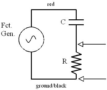
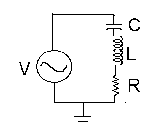
These frequency-dependent effects of inductor and capacitors can be useful in a variety of ways. One is separating high frequency signals from low frequency ones. This might be useful, for example, if you wanted to reduce a 120 Hz hum in your radio. You could use a resistor in series with a capacitor as shown below. The output connection is shown by the arrows.
The capacitor and resistor form a frequency dependent voltage divider - i.e. the voltage across the resistor (output voltage) will change as the frequency changes. At low frequencies the reactance of the capacitor, XC, is large causing the current to be small. A small current flowing through a resistor causes only a small voltage, however a small current flowing through a large capacitive reactance causes a large voltage across the capacitor. Thus, you measure a very small voltage (across the resistor) for low frequencies. At high frequencies XC will be much smaller than the value of the resistor. The current will be larger, giving a significant output voltage for high frequencies. So low frequency hum will be reduced without too much alteration of the higher frequencies. The circuit shown above is called a R-C High Pass filter. You should think through the case where the output is measured across the capacitor - what will be its frequency behavior? (Hint: this sounds like a lab quiz question).
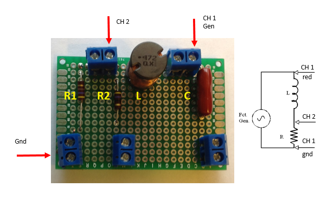
We will now investigate a L-R filter. All of the components for this experiment have been mounted on a circuit board for convenience as shown below along with its schematic and component values.
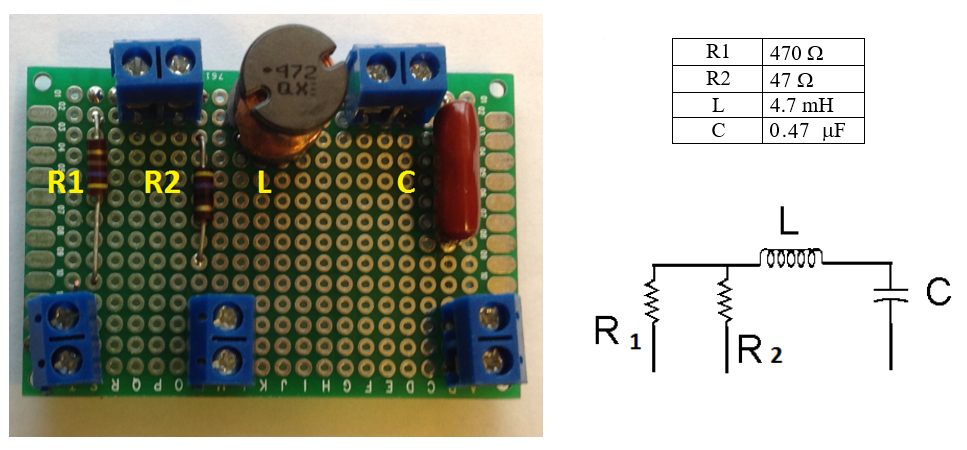
Connections are made to the blue blocks. Both of the screw terminals are connected together in each block. There may be short wires attached to the blocks to allow you to make connections more easily.
When this lab used analog oscilloscopes the process of taking data was pretty involved. Once you had the waveform displayed, you had to use the the Horizontal Position to shift the trough of the waveform to the center vertical line with the fractional division marks. This value was recorded and the Horizontal Position was again used to shift the crest of the waveform to the center line and that value was recorded. The two values were subtracted and then multiplied by the number of V/div to obtain the peak-to-peak voltage. This had to be done for both the input and the output voltage of the circuit - a time consuming process that will be mostly automated for you.
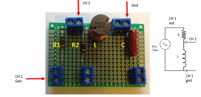
Part I. Set up the circuit shown below using the inductor and R1.
We want to experimentally determine the Transfer Function, i.e. the fraction of the input voltage that is observed at the output. With the oscilloscopes that were used in the past, that meant adjusting generator to set the CH 1 value before each measurement. Our DSO knows how to measure a voltage pretty accurately so we will just set the generator output and have the DSO measure both CH1 and CH2 for us. For our experiments the transfer function is the voltage in channel 2 divided by the voltage in channel 1.
Set up your DSO as shown below.
| Use your oscilloscope Channel 1 to monitor the voltage from the generator (input voltage or Vgen) |
| Use Channel 2 to measure the voltage across the inductor (output voltage or VL) |
| Set your function generator for a frequency of 7.5 kHz, sine wave, |
| Set the Function Generator for 2 volts, peak to peak. You may find that 0.500 V/div is a convenient value for the volts/division for Ch1 as 2Vpp will fill 4 of the 8 vertical blocks. |
| Turn the function generator output ON and adjust your Time/div and Volts/div to obtain a trace that shows 2 or 3 cycles. |
For CH 1 and CH 2 measure the position of the trough on the center axis and the position of the crest on the center axis as described above. Subtract the two to find the peak-to-peak number of divisions and calculate the peak to peak input voltage. Complete the table with your data and calculations
| Ch 1 Trough | Ch 1 Crest | Difference | V/div | Ch 1 Voltage | Ch 2 Trough | Ch 2 Crest | Difference | V/div | Ch 2 Voltage | Transfer Fct |
Fortunately, your DSO knows how to measure peak-to-peak voltages. Press the 'Measure' button. Press the topmost 'Soft Key' until Ch2 is displayed. Press 'Voltage' and choose peak-to-peak. Then turn off the menu. You should have a numerical value of the peak-to-peak voltage displayed in the same color as the trace of Channel 2. Repeat for Ch 1. Compare the DSO's values with those you determined above for the Voltage. Do they agree? If not, attempt to explain why. If you have a serious discrepancy, ask your instructor for help.
The next part of this investigation will measure Vin and Vout for a number of frequencies. In the past, you had to perform all of the measurements by hand. With the DSO, we can use a computer program to take the data for us - which will allow more time for analysis and reflection.
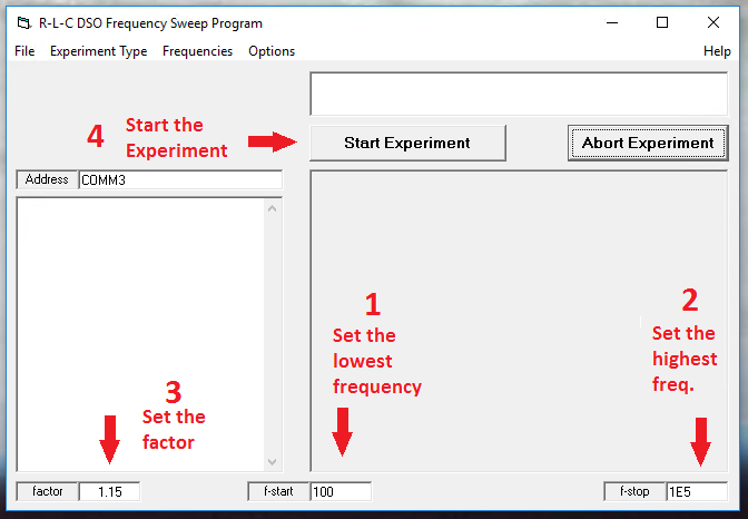
Double Click the 'DSO_Sweep' shortcut on the desktop. A program will start as shown below. Red arrows and notes have been added. Once started, the program will set the generator frequency in the DSO to f-start and then measure Ch 1 and Ch 2 voltages. Next it will multiply the frequency by the factor (100 x 1.15 = 115 Hz for the second point for the default values). The process is continued until the frequency is larger than f-stop. The white area above the 'Start Experiment' button will tell you what the program is doing. When the experiment has finished or after 'Abort Experiment' has been clicked the box will say 'Done'. The graph that shows up as the data is taken is the Ch. 2 Voltage (output). The white area above the 'factor' will have a set of data in the order of frequency, Ch 1, and Ch 2. Once the white area above 'Start Experiment' says 'Done' you can right click in the text area then choose 'select all'. Then right click again and choose 'Copy' to copy the data to the clipboard. The data can be pasted directly into a data table in Logger Pro or Graphical Analysis for further analysis and printing.
Use the default values in the program and click on 'Start Experiment' at this time. Once the program has finished, copy the data using the steps above. It is not necessary to close the program at this time.
Logger Pro will be used to perform the computations and plot the data. Start Logger Pro and begin by adding changing the names of the columns as showing below. Next add a manual column and name it Vout.| Freq. (Hz) | Vin (V) | Vout (V) |
Then paste your data into the uppermost frequency in the table. All three columns should be filled in.
Complete the following table by adding a calculated column. The Transfer Function is just Vout / Vin. Once the entire table is completed, plot a graph of the Transfer Function (Vout/Vin) as a function of the frequency, F.
| Freq. (Hz) | Vin (V) | Vout (V) | TF = Vout/Vin |
When plotted with linear axes, you will find that the data for most of the frequencies you measured is very compressed near the left side of the graph. Plot a second graph using a logarithmic scale of the frequency for your horizontal axis. (There is a check box for 'Log Axis' just above the 'Help' button in the 'Axis Options' tab of 'Graph Options.) Comment on the appearance of your graph afterwards. Finally make a plot of the Transfer Function versus Frequency with the 'Log Axis' box checked for the y-axis. Include this graph and your data table in your notebook. Save your experiment as RL1.cmbl. If a file already exists, overwrite it.
The transfer function is the ratio of Vout / Vin as a function of frequency. It represents the fraction of the input delivered to the output of the circuit. Based on your final graph, would you characterize the circuit to be a high pass, low pass or band-pass filter? Explain.
Next, reverse the ground and Ch1 connections to give the circuit shown in the diagram below.
Go back to 'DSO_Sweep' and take another set of data. Once the program is done, select and copy your data as before. If you did not change factor, f-start or f-stop, you can just paste your data into the topmost frequency and everything will be recalculated automatically. Print your data table and the plot of the Transfer Function versus Frequency with the 'Log Axis' checked for both axes and include them in your report. Save your experiment as RL2.cmbl. If a file already exists, overwrite it.
How does the filter action of this circuit compare to your first circuit? Explain.
In the final graph you should have observed a plot with two linear regions that would intersect to form a 'corner' if they were extended. Determine the approximate frequency of the corner, fc. Theory tells us that the corner frequency, fc, and time constant, t (tau), should obey 2p(fc)(t) = 1. Check to see that this is approximately correct. Comment on the agreement.
Set up the circuit shown below using resistor R1 = 470 ohms. Ground goes to the free end of R1. CH 2 goes to the junction between the resistors and the inductor, and CH1/Gen goes to the free end of the capacitor.
Using the same input voltage and frequencies as in Part I, measure the voltages necessary to calculate the transfer function. You will again be running 'DSO_Sweep'. You should be able to paste your results into the topmost frequency and have the values automatically recalculated. Plot TF versus Frequency with the 'Log Axis' box checked on the x-axis and unchecked for the y-axis. Your plot should have a peak. Print your data table and the plot for inclusion with your report. Save your experiment as RLC1.cmbl. If a file already exists, overwrite it.
Next move the ground connection to the free end of R2 and repeat the process, including the printing for your report. How was your graph affected by changing the resistance? Explain.
We need more data around the frequency of peak output. Use your cursor to measure the approximate frequencies at which the amplitude of the Transfer Function is about 50% of the maximum value. Use these frequencies as f-start and f-stop. Set the factor around 1.03. Take another set of data and add that data to your existing plot by pasting it into the first empty Frequency in your data table. Use the 'Sort' function in the 'Data' menu to put the data in frequency order (not necessary if you do not connect the points with lines). Include your data table and this plot in your lab report. Save your experiment as RLC2.cmbl. If a file already exists, overwrite it.
The frequency of maximum output is called the resonant frequency of the series R-L-C circuit. Using your graph carefully estimate the frequency of the peak's center. This is the experimental resonant frequency. Calculate the theoretical resonant frequency for your circuit and compare it to your experimental value. (hint: In lecture you learned that the inductive reactance is numerically equal to the capacitive reactance at the resonant frequency.)
Try to explain why the width of the resonance peak differs for the two values of the resistance that were used. Explain.