Filters and Resonant Circuits
Last week you observed the effect that capacitors have on the current in a circuit that was essentially a switched DC circuit. Today you will extend your observations to AC circuits and look at the effects of inductors as well.
In a DC circuit, there is only current until the capacitor is fully charged. However, in an AC circuit of high enough frequency the capacitor never has time to get fully charged before the voltage reverses causing the capacitor to discharge. Thus, there is always current in the circuit. An inductor has little effect other than adding resistance to a DC circuit because it is basically just a long piece of wire. However, the rapidly changing currents of AC set up magnetic fields which, according to Faraday's Law, lead to induced emf in the coil which always opposes the original current change. The more rapidly the current changes (high frequency AC) the greater will be the induced opposition.
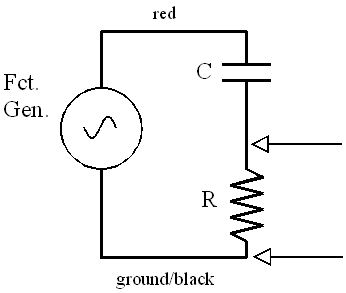
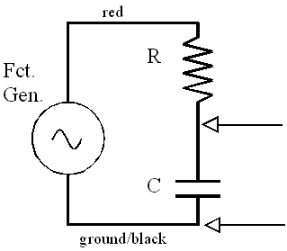
These frequency-dependent effects of inductor and capacitors can be useful in a variety of ways. One is separating high frequency signals from low frequency ones. This might be useful, for example, if you wanted to get rid of a 60-Hz hum in your radio. You could use a capacitor or inductor in series with a resistor as shown below. Consider the RC circuit (top left picture). If the input voltage voltage has a high frequency, then the capacitor never has a chance to develop much charge and its voltage will be low. Thus, the voltage across the resistor will be almost equal to the input voltage. On the other hand, if the frequency is low, the charging happens slowly, so that most of the time the capacitor is fully charged. Then I ~ 0 and so will be the voltage across the resistor. Thus, you measure a significant output voltage for high frequencies. You should think through the other three cases for yourself. (Hint: this sounds like a lab quiz question).
|
|
|
| R-C High Pass | R-C Low Pass |
|
|
|
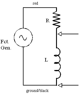
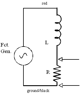
| R-L High Pass | R-L Low Pass |
By combining a capacitive high pass filter in series with an inductive low pass filter, you can make a resonant circuit, which selects a band of frequencies to pass, while reducing the amplitude of frequencies that are higher or lower. Such circuits were used for tuning a radio to a particular station.
When this lab used analog oscillopes the process of taking data was pretty involved. Once you have the waveform displayed, you had to use the the Horizontal Position to shift the bottom of the waveform to the center vertical line with the fractional division marks. This value was recorded and the Horizontal Position was again used to shift the top of the waveform to the center line and that value was recorded. The two values were subtracted and then multiplied by the number of V/div to obtain the peak-to-peak voltage.
Part I. Set up the circuit shown below with R = 4700 ohms and C = 0.01 microfarad.
| Use your oscilloscope Channel 1 to monitor the voltage from the generator (input voltage or Vgen) |
| Use Channel 2 to measure the voltage across the capacitor (output voltage or Vcap) |
| Set your function generator for a frequency of 7.5 kHz, sine wave, |
| Set the Function Generator for 2 volts, peak to peak. You may find that 0.500 V/div is a convenient value for the volts/division for Ch1 as 2Vpp will fill 4 of the 8 vertical blocks. |
| Turn the function generator output ON and adjust your Time/div and Volts/div to obtain a trace that shows 2 or 3 cycles. |
Using the technique described for analog scopes above, measure the position of the trough on the center axis, the position of the crest on the center axis. Subtract the two to find the peak-to-peak number of divisions and calculate the peak to peak output voltage. Record the data and calculations in your lab notebook.
Fortunately, your DSO knows how to measure peak-to-peak voltages. Press the 'Measure' button. Press the topmost 'Soft Key' until Ch2 is displayed. Press 'Voltage' and choose peak-to-peak. Then turn off the menu. You should have a numerical value of the peak-to-peak voltage displayed in the same color as the trace of Channel 2.
The next part of this investigation will measure Vin and Vout for a number of frequencies. Logger Pro will be used to perform the computations and plot the data. Measure the input and output voltage at each of the following frequencies in the following table and complete the table. You will need to adjust the Time/div as you change the frequency and to change the V/div on Ch2 to keep the displayed value sufficiently large as to yield good data - a minimum of 3 Div peak-to-peak is recommended.
| Gen. Freq. | Vout (V) | Vin (V) |
| 20 Hz | ||
| 50 Hz | ||
| 100 Hz | ||
| 200 Hz | ||
| 500 Hz | ||
| 1 kHz | ||
| 2 kHz | ||
| 5 kHz | ||
| 10 kHz | ||
| 20 kHz | ||
| 50 kHz | ||
| 100 kHz | ||
| 200 kHz |
Complete the following table and compute the ratio of Vcap / Vgen (which is also referred to as Vout / Vin). Once the entire table is completed, plot Vout/Vin as a function of the frequency, F.
| Gen. Freq. | Vout (V) | Vin (V) | F (Hz) | Log(F) | Vout/Vin | Log(Vout/Vin) |
You will find that the data for most of the frequencies you measured is very compressed near the left side of the graph. Plot a second graph using log(F) instead of the frequency for your horizontal axis. Finally make a plot of Log(Vout / Vin) versus Log(F) and include it and your data table in your notebook.
The ratio of Vout / Vin as a function of frequency is called the transfer function. It represents the fraction of the input delivered to the output of the circuit. Based on your final graph, would you characterize the circuit to be a high pass, low pass or band-pass filter? Explain.
In the final graph you should have observed a plot with two linear regions that would intersect to form a 'corner' if they were extended. Determine the approximate frequency of the corner, fc. Theory tells us that the time constant should be equal to 1/(2pfc). Check to see that this is approximately correct.
Part II. Set up the circuit shown below with R = 1000 ohms, C = 0.1 microfarad and L = 2.5 milliHenry. Keep Ch1 on the function generator and Ch2 across the resistor.
Using the same input voltage and frequencies as in Part I, measure the voltage across the resistor. Be sure to change you Volts/Div on Ch2 as necessary to keep good data as described earlier.
| Gen. Freq. | Vout (V) | Vin (V) |
| 20 Hz | ||
| 50 Hz | ||
| 100 Hz | ||
| 200 Hz | ||
| 500 Hz | ||
| 1 kHz | ||
| 2 kHz | ||
| 5 kHz | ||
| 10 kHz | ||
| 20 kHz | ||
| 50 kHz | ||
| 100 kHz | ||
| 200 kHz |
Once you have your raw data use Logger Pro to compute the quantities in a table with the following columns.
| Gen. Freq. | Vout (V) | Vin (V) | F (Hz) | Log(F) | Vout/Vin |
Plot Vout/Vin versus log(Frequecy). Your plot should have a peak. Once you have identified the frequency of peak output take some more data near this frequency trying to locate the frequency which gives you the maximum output. Add the additional points to your table and plot. Include your data table and this plot in your lab report.
The frequency of maximum output is called the resonant frequency of the series R-L-C circuit. Calculate the theoretical resonant frequency for your circuit and compare it to your experimental value. (hint: In lecture you learned that the inductive reactance is numerically equal to the capacitive reactance at the resonant frequency.)
If time permits, replace the 1000 ohm resistor with a 47 ohm resistor and explore the region around the resonant frequency. You might find a new table and plot helpful. Is the shape of the peak around resonance the same, more broad or more narrow than before? Explain.